One option for implementing a dynamic cost surface is to use a continuously updated network, where the latest available data at the starting time of travel is used, and where the cost of travel does not change during the duration of the estimated route. Another option is to establish a network with varying travel cost per pre-defined time interval. In this case the travel cost is dependent on the starting time of travel, and the travel cost changes when the estimated route passes from one time interval to another.
In practice, the first approach involves building an application that passes on values to the cost surface used in a raster-based GIS for calculating the fastest path in a network. The second approach involves working with multiple cost surfaces for estimating the fastest path, which is the one that will be used here.
This approach uses an average cost-of-passage surface for each time interval. If one-hour time intervals were used, one would need 24 cost surfaces to cover a 24-hour period.
Applied within the context of time intervals, the first proximity surface is cut off when the time interval border is traversed. Then, from all endpoints, new proximity surfaces and shortest paths are calculated, until the destination is reached. Computationally this can turn into a considerable task, depending on the number of time intervals traversed and the number of paths generated in each time interval: If time interval A yields 4 possible paths from a starting point, then for time interval B, the four paths must be continued until the destination or a new time interval is reached. When the destination has been reached the values of all paths must be added and compared. In practice, one must calculate proximity surfaces from a starting point to cut-off points where a new time interval begins, and from cut-off points to starting point, adding the surfaces yields the accumulated cost-of-passage (time) value for each path. Then, from each cut-off point the procedure has to be repeated until destination or a new time interval is reached. Finally the accumulated cost-of-passage value for each successively linked path must be calculated and compared to find the path with the lowest accumulated value.
In detail, the steps would be as follows:
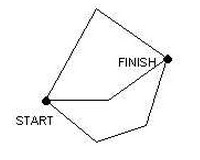
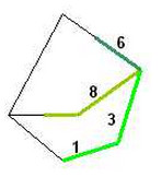
Input: A network, with 3 possible ways from starting point to destination point.
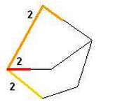
Step1: Spread from starting point, cut-off when accumulated cell values indicate that a time interval borderline is being passed. Then, spread backwards from the cut-off points to starting point. Adding the proximity surfaces yields the cost-of-passage for this time interval for the various paths.
Step 2: For all cut-off points, spread until next time interval or (in this case) until the destination has been reached. Spread backwards from destination and add proximity surfaces to yield the cost-of-passage values for all possible paths. Retain the paths from the cut-off points to destination that have the lowest cost-of-passage.
Discard other paths
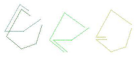
Step 3: Add the cost-of passage for the partial paths to yield the final cost-of-passage value for the remaining paths.
Retain the path with the lowest value.