Supply Chain Risk. Business Continuity. Transport Vulnerability. Resilience. Articles and papers. Books and book chapters. Reports and whitepapers. And more.
Usually, to generate a cost-of passage surface, several variables will be collapsed into one layer. These variables might be road class, average speed, traffic density, and congestion during specific time of day or other factors that contribute to the overall cost variable. The cost-of-passage surface can be defined by a variety of measurement units: time, fuel consumption, money or other possible cost units, for which the least cost passage is to be determined.
Using average speed and time as a means of inferring cost-of-passage is among the most common approach in network analysis, since it is easy to use and calculate. However, “least cost” does not always need to be “least time”; it may just as well be least fuel, least length, or any least cost variable that can be implemented in a cost-of-passage surface.
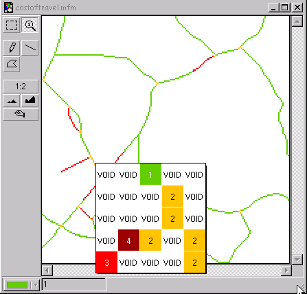
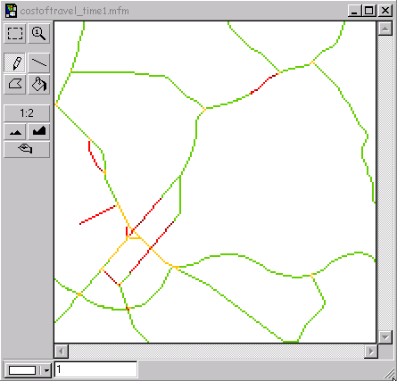
Cost surface, with values indicating impedance to travel (cost) across the cells.
One option for implementing a dynamic cost surface is to use a continuously updated network, where the latest available data at the starting time of travel is used, and where the cost of travel does not change during the duration of the estimated route. Another option is to establish a network with varying travel cost per pre-defined time interval. In this case the travel cost is dependent on the starting time of travel, and the travel cost changes when the estimated route passes from one time interval to another.
In practice, the first approach involves building an application that passes on values to the cost surface used in a raster-based GIS for calculating the fastest path in a network. The second approach involves working with multiple cost surfaces for estimating the fastest path, which is the one that will be used here.
This approach uses an average cost-of-passage surface for each time interval. If one-hour time intervals were used, one would need 24 cost surfaces to cover a 24-hour period.
Applied within the context of time intervals, the first proximity surface is cut off when the time interval border is traversed. Then, from all endpoints, new proximity surfaces and shortest paths are calculated, until the destination is reached. Computationally this can turn into a considerable task, depending on the number of time intervals traversed and the number of paths generated in each time interval: If time interval A yields 4 possible paths from a starting point, then for time interval B, the four paths must be continued until the destination or a new time interval is reached. When the destination has been reached the values of all paths must be added and compared. In practice, one must calculate proximity surfaces from a starting point to cut-off points where a new time interval begins, and from cut-off points to starting point, adding the surfaces yields the accumulated cost-of-passage (time) value for each path. Then, from each cut-off point the procedure has to be repeated until destination or a new time interval is reached. Finally the accumulated cost-of-passage value for each successively linked path must be calculated and compared to find the path with the lowest accumulated value.
In detail, the steps would be as follows:
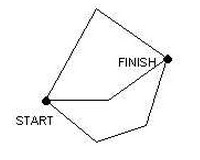
Input: A network, with 3 possible ways from starting point to destination point.
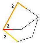
Step1: Spread from starting point, cut-off when accumulated cell values indicate that a time interval borderline is being passed. Then, spread backwards from the cut-off points to starting point. Adding the proximity surfaces yields the cost-of-passage for this time interval for the various paths.
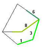
Step 2: For all cut-off points, spread until next time interval or (in this case) until the destination has been reached. Spread backwards from destination and add proximity surfaces to yield the cost-of-passage values for all possible paths. Retain the paths from the cut-off points to destination that have the lowest cost-of-passage.
Discard other paths
Step 3: Add the cost-of passage for the partial paths to yield the final cost-of-passage value for the remaining paths.
Retain the path with the lowest value.
Map layers needed: A network, a cost surface, origin and destination point,
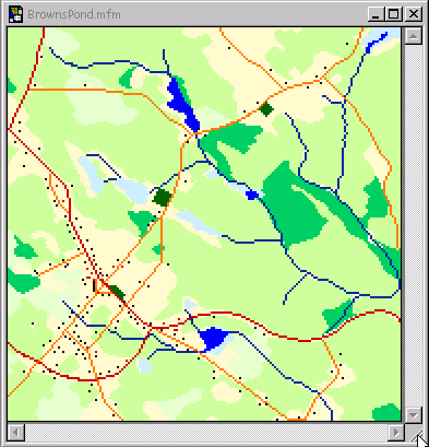
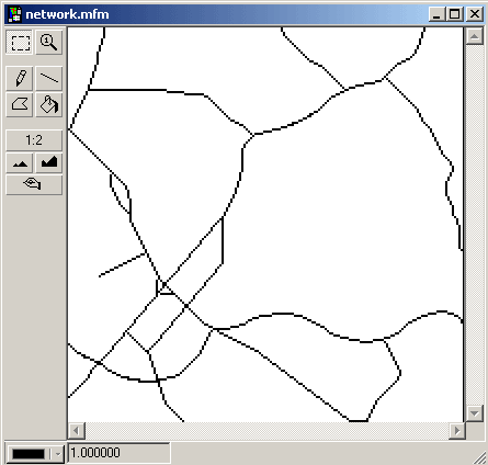
network.mfm
costoftravel.mfm
startstop.mfm
(image missing)
The network is a replica of the Brown’s Pond study area used by Tomlin. The cost surface are fictitious values, 1-4, indicating impedance. Origin and destination were derived by assigning the values 999 and 998 respectively to points on the network map (startstop.mfm) and then extracting each point using Recode.
Necessary cookies help make a website usable by enabling basic functions like page navigation and access to secure areas of the website. The website cannot function properly without these cookies.
We do not use cookies of this type.
Marketing cookies are used to track visitors across websites. The intention is to display ads that are relevant and engaging for the individual user and thereby more valuable for publishers and third party advertisers.
We do not use cookies of this type.
Analytics cookies help website owners to understand how visitors interact with websites by collecting and reporting information anonymously.
We do not use cookies of this type.
Preference cookies enable a website to remember information that changes the way the website behaves or looks, like your preferred language or the region that you are in.
We do not use cookies of this type.
Unclassified cookies are cookies that we are in the process of classifying, together with the providers of individual cookies.
We do not use cookies of this type.
Cookies are small text files that can be used by websites to make a user's experience more efficient. The law states that we can store cookies on your device if they are strictly necessary for the operation of this site. For all other types of cookies we need your permission. This site uses different types of cookies. Some cookies are placed by third party services that appear on our pages.