Supply Chain Risk. Business Continuity. Transport Vulnerability. Resilience. Articles and papers. Books and book chapters. Reports and whitepapers. And more.
These pages will explain how to do network analysis in raster GIS using MFworks as an example software. MFworks has evolved from MAPFactory, originally designed by C. Dana Tomlin, the father of map algebra. This is unmistakably seen in MFworks command procedures and scripting language. MFworks is thus the ideal companion for teaching and learning Tomlin’s principles of map algebra. MFWorks was featured in a very positive review in the June 2000 edition of GeoEurope as the only raster GIS truly capable of network analysis. I decided to put that statment to the test.
MFworks
Conducting network analysis in MFworks comprises iterative steps that lead to a functioning network. These steps will convert map layers with square cells into linear elements that are linked together as lines, with directional flows assigned to each cell, and map layers containing cost variables. This example, based on my MSc in GIS, will show how network analysis is performed in MFworks, both with a fixed travel cost for the entire time of travel and with a dynamic travel cost, where the cost of travel changes during the time of travel.
The key to producing a successful network model is in understanding the relationship between the characteristics of physical network systems and the representation of those characteristics by the elements of the network model. The efficacy and validity of the network depends on how precisely the network can be modeled to match the real world network it represents. A network can be explicitly modeled in vector GIS, but can only be approximated by a raster GIS like MFworks.
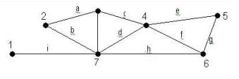
Network representation in vector GIS: Nodes (numbers) and arcs (letters)
A network in vector GIS takes the form of edges (or arcs) connecting pairs of nodes (or vertices). Nodes can be junctions and edges can be segments of a road. For a network to function as a real-world model, an edge will have to be associated with a direction and with a measure of impedance, determining the resistance or travel cost along the network.
Even if it does not appear so explicitly, a grid made up of cells in a raster GIS is in fact a graph representing a network, with 8 possible directions from each node. However, the grid cells only approximate the exact shapes of the lines in the network. Also, the direction is not as explicitly given as in the vector model. Thirdly, the line and node attributes must be stored as a separate layer for each attribute. As a result, a network using a raster model normally consists of a vast number of layers. Since the grid has a given resolution, the cells will only approximate the exact length of the network.
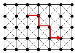
Tracing a path from cell to cell in raster GIS
generates a zigzag path instead of a straight line.
Using Tomlin’s Incremental Length, Incremental Linkage, and Directional Identifiers, which identify underlying linear features, MFworks makes it possible to model a road network in raster GIS in much the same manner as in vector GIS. The first step is to extract linear features from neighboring raster cells; the second step is to assign directions.
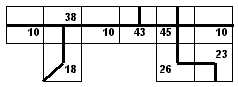
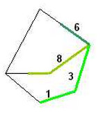
This operation infers the lineal characteristic of raster cells, by equating consecutive locations with a set of straight lines between them (Figure 1-3). Based on its relations with neighboring cells that have the same attribute value, each cell is given a linkage value indicating how it is linked to other cells.
By assigning a value to each cell equivalent to the linear feature it represents it is possible to create a network similar to a road network. The smaller the cell resolution, the better the real-world road network will be approximated by this procedure.
Building a road network using Incremental Linkage from
figure 1-3 with cell values representing linear features
The second step to creating a road network in raster GIS is to impose constraints on the flow that can take place from cell to cell.
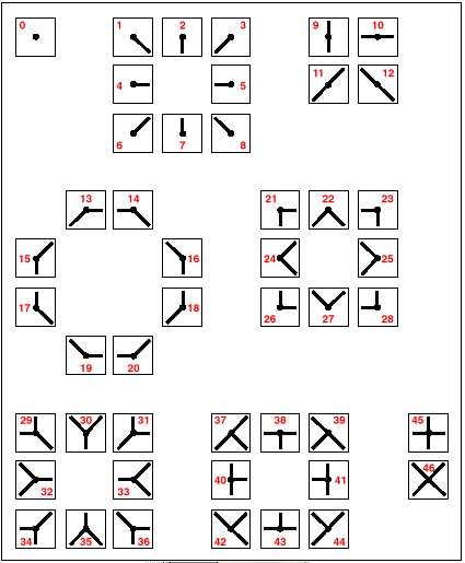
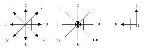
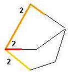
The second step to creating a road network in raster GIS is to impose constraints on the flow that can take place from cell to cell. The value assigned to the centre cell in a 3×3 window indicates the directions the flow can take in and or out of this cell. Figure 1-5 shows how a cell value of 10 is inferred from flow in direction 8 and 2.
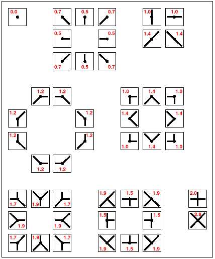
Tomlin’s directional identifiers: Cell values indicate possible flow direction in or out of cell
The directional identifiers that are to be assigned to any given cell in a road network can be directly inferred from the Incremental Linkage values, i.e. Incremental Linkage value 28 yields directional constraints value 10, and so on. The transition from Incremental Linkage to Directions is done through a straightforward reassigning of the cell values in the Incremental Linkage map layer to corresponding values in the Directions map layer. More specific constraints, like one-way directions or dead-end roads, which are not directly inferable from the mentioned linkage values, will have to be assigned manually.
Inferring flow directions from Incremental Linkage values in figure above
Usually, to generate a cost-of passage surface, several variables will be collapsed into one layer. These variables might be road class, average speed, traffic density, and congestion during specific time of day or other factors that contribute to the overall cost variable. The cost-of-passage surface can be defined by a variety of measurement units: time, fuel consumption, money or other possible cost units, for which the least cost passage is to be determined.
Using average speed and time as a means of inferring cost-of-passage is among the most common approach in network analysis, since it is easy to use and calculate. However, “least cost” does not always need to be “least time”; it may just as well be least fuel, least length, or any least cost variable that can be implemented in a cost-of-passage surface.
Cost surface, with values indicating impedance to travel (cost) across the cells.
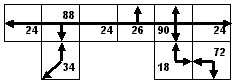
To determine the actual length of a path through a number of cells the Incremental Length operation is used. Incremental Length works similar to Incremental Linkage to the extent that Incremental Linkage is used implicitly to determine the linkage, from which the length is inferred. Incremental Length then applies the factor by which the cell resolution has to be multiplied to yield the length of the linear features in any cell.
It should be noted that Incremental Length calculates the factor for inferring the total length of all linear features in any cell. When uncritically applied to deriving the time of traversing a cell, this function may not yield exact results, since the time of passing straight through a cell may differ from the calculated value, which takes into account all linear features in that cell, even those that are not traversed. The smaller the cell resolution and the higher the average speed, the more negligible this error becomes.
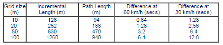
Assessing discrepancy between actual path length
and length inferred from Incremental Linkage
The figure and table above demonstrates an example of this “error”. The bold line is the path sought; the shaded cells indicate where the Incremental Length factor deviates from the actual length. The table shows how cell resolution and average speed influence the magnitude of the error.
To determine the length of a particular road stretch, this stretch first has to be separated, then made subject to the Incremental Length operator to find the correct length. Whether this last procedure is absolutely necessary will depend on the cell resolution and whether deriving the actual path length is strictly required as a result of the task in question.
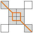
A special case, illustrating the discrepancy between inferred and actual path length, as described previously, appears at crossroads and junctions and deserves particular attention, especially at non-90-degrees junctions, as shown in the following example:
Sought path through a junction
The actual path sought is a straight line through the junction, indicated by the shaded cells. The bold lines indicate the actual linear features. Here, the actual path length is cell resolution x 5.6 (1.4 x 4).
Inferred path, as result of Incremental Length/ Incremental Linkage
In order to justify the inferable directions, the Incremental Length operator will link to many cells together, as shown by the shaded cells and bold line. The inferred path is equal to cell resolution x 8.2 (1.7 x 2 + 1.4 x 2 + 1 x 2), thus overestimating the actual path over this section by 2.6 x cell resolution. Unless there is substantial difference in cost-of-passage between the two roads that cross each other, which then prohibits the off-path cells from being included in the added proximity surfaces, this error will occur in most cases with such junctions.
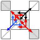
Correctly modelled junction, linkage indicated by bold lines, direction indicated by arrows
A solution to avoid this from the beginning, before finding the least-cost path, would be to model the linkage correctly, and allow the direction to flow differently. The fact that it is possible to completely detach the direction of the flow in a network from the underlying linear feature is indeed an interesting observation concerning the modeling of networks in raster GIS.
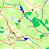
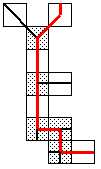
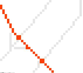
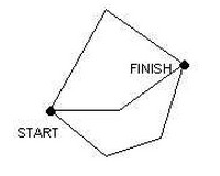
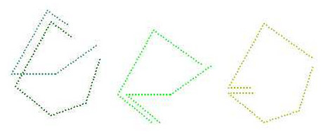
The above can also be demonstrated by an example from the study area. Note the linked square in the left image, as opposed to the straight line in the right image:
(a) Least-cost path using generically inferred directions
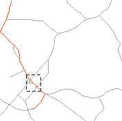
(b) Location of a and c in study area
(c) Least-cost path using manually inferred directions
One option for implementing a dynamic cost surface is to use a continuously updated network, where the latest available data at the starting time of travel is used, and where the cost of travel does not change during the duration of the estimated route. Another option is to establish a network with varying travel cost per pre-defined time interval. In this case the travel cost is dependent on the starting time of travel, and the travel cost changes when the estimated route passes from one time interval to another.
In practice, the first approach involves building an application that passes on values to the cost surface used in a raster-based GIS for calculating the fastest path in a network. The second approach involves working with multiple cost surfaces for estimating the fastest path, which is the one that will be used here.
This approach uses an average cost-of-passage surface for each time interval. If one-hour time intervals were used, one would need 24 cost surfaces to cover a 24-hour period.
Applied within the context of time intervals, the first proximity surface is cut off when the time interval border is traversed. Then, from all endpoints, new proximity surfaces and shortest paths are calculated, until the destination is reached. Computationally this can turn into a considerable task, depending on the number of time intervals traversed and the number of paths generated in each time interval: If time interval A yields 4 possible paths from a starting point, then for time interval B, the four paths must be continued until the destination or a new time interval is reached. When the destination has been reached the values of all paths must be added and compared. In practice, one must calculate proximity surfaces from a starting point to cut-off points where a new time interval begins, and from cut-off points to starting point, adding the surfaces yields the accumulated cost-of-passage (time) value for each path. Then, from each cut-off point the procedure has to be repeated until destination or a new time interval is reached. Finally the accumulated cost-of-passage value for each successively linked path must be calculated and compared to find the path with the lowest accumulated value.
In detail, the steps would be as follows:
Input: A network, with 3 possible ways from starting point to destination point.
Step1: Spread from starting point, cut-off when accumulated cell values indicate that a time interval borderline is being passed. Then, spread backwards from the cut-off points to starting point. Adding the proximity surfaces yields the cost-of-passage for this time interval for the various paths.
Step 2: For all cut-off points, spread until next time interval or (in this case) until the destination has been reached. Spread backwards from destination and add proximity surfaces to yield the cost-of-passage values for all possible paths. Retain the paths from the cut-off points to destination that have the lowest cost-of-passage.
Discard other paths
Step 3: Add the cost-of passage for the partial paths to yield the final cost-of-passage value for the remaining paths.
Retain the path with the lowest value.
Using raster GIS for network analysis leads into a simplification of a complex network structure. The path is prone to be distorted, firstly, due to the mistaken length introduced by Incremental Length, and secondly, due the zigzagged path, a consequence of the innate grid structure. Nonetheless, a fine-tuned use of Incremental Linkage and a minimal cell resolution can have a smoothing effect on the exact delineation of the path. On the other hand, minimising cell resolution increases computation.
In raster GIS the precision of the model is determined by the cell resolution, the finer the resolution (the smaller the cell size), the better the precision. For this research a cell resolution of 20m was deemed appropriate for the task in question, as it would allow encompassing normal road width and adjacent areas within one cell width. For a dense inner city road network a cell resolution of 10m would be preferable, allowing even narrow blocks to be incorporated into the model.
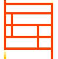
The infamous multiple path problem
The concept of adding proximity surfaces will some times lead to peculiar artefacts. A special case appears in a regular lattice if the cost surface is isotropic: Here the multiple path problem is clearly visible, since all possible paths per se have the same accumulated cost towards the destination. Here, human mind, as opposed to computer mind, would intuitively seek out a solution that implements a heuristic search, always following the path that yields the shortest Euclidian distance to the destination.
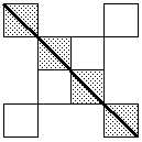
Multiple path problem in regular lattice with homogenous cost surface. Start at top left, destination at bottom right.
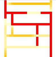
More often occurs the so-called multiple path problem, particularly if the road network and the cost surface are oversimplified. There are no distinctive low values, so that in order to gain a coherent route from start to destination so many low valued cells have to be selected that no clear path can be discerned.
Typical multiple path problem. Start at top left, destination at bottom right.
Map layers needed: A network, a cost surface, origin and destination point,
network.mfm
costoftravel.mfm
startstop.mfm
(image missing)
The network is a replica of the Brown’s Pond study area used by Tomlin. The cost surface are fictitious values, 1-4, indicating impedance. Origin and destination were derived by assigning the values 999 and 998 respectively to points on the network map (startstop.mfm) and then extracting each point using Recode.
This operation converts linkage values into directional values.
direction_raw = Recode linkage
Assigning 128 to 1
Assigning 64 To 2
Assigning 32 To 3
Assigning 16To 4
Assigning 8 To 5
Assigning 4 To 6
Assigning 2 To 7
Assigning 1 To 8
Assigning 66To 9
Assigning 24 To 10
Assigning 36 To 11
Assigning 129 To 12
Assigning 48 To 13
Assigning 136 To 14
Assigning 68 To 15
Assigning 65 To 16
Assigning 130 To 17
Assigning 34 To 18
Assigning 17 To 19
Assigning 12 To 20
Assigning 80 To 21
Assigning 160 To 22
Assigning 72 To 23
Assigning 132 To 24
Assigning 33 To 25
Assigning 18 To 26
Assigning 5 To 27
Assigning 10 To 28
Assigning 138 To 29
Assigning 69 To 30
Assigning 50 To 31
Assigning 49 To 32
Assigning 140 To 33
Assigning 76 To 34
Assigning 162 To 35
Assigning 81 To 36
Assigning 164 To 37
Assigning 88 To 38
Assigning 161 To 39
Assigning 82 To 40
Assigning 74 To 41
Assigning 133 To 42
Assigning 26 To 43
Assigning 37 To 44
Assigning 90 To 45
Assigning 165 To 46
;
The direction_raw map must now be edited to make sure that the shortest path is found, particularly in intersections and junctions. The actual editing depends on the real network
(road) features, see travel cost and path length.
direction = manual edit of direction_raw
The edited values are displayed in color in the directions map, unedited cells are in grayscale.
The shortest path is delineated by the cells with the lowest value(s). The value is the actual cost of using this path. Using the Legend function this path can be derived by changing the color of the cells with the lowest value until a continuous path from origin to detination can be seen.
ShortestPath = Recode ShortestPath_InNetwork
Assigning 999 To 262…264;
262-264 were the cell values for the shortest path. A high value of 999 was the chosen for the path to distinctively separate the path cells from any other cells in the following overlay:
The extracted path can be overlayed over the study area map for visualization.
ShortestPath_OverMap = Cover BrownsPond With ShortestPath ;
The procedure is similar to finding the shortest path through a network with no time-dependent travel cost.
First calculate the path(s) from origin to the cutoff-point(s), where the new time interval starts. In other words spread until the available time in time interval 1, depending on your starting time, has been used up. From the cutoff-point(s) in time interval 1, calculate the shortest path(s) to the destination through time interval 2. The path with the lowest value is the sought path. Join the paths.
The cell value at the cutoff-point for time interval 1added to the cell values of the shortest path in time interval 2 is the total cost for the joined path.
If using 3 time intervals, repeat the procedure for time interval 1 in time interval 2. If using 4 time intervals, repeat the procedure for time interval 2 in time interval 3, and so forth.
See the theory behind it.
The procedure is similar to finding the shortest path through a network with no time-dependent travel cost (go there first).
First calculate the path(s) from origin to the cutoff-point(s), where the new time interval starts. In other words spread until the available time in time interval 1, depending on your starting time, has been used up. From the cutoff-point(s) in time interval 1, calculate the shortest path(s) to the destination through time interval 2. The path with the lowest value is the sought path. Join the paths.
The cell value at the cutoff-point for time interval 1added to the cell values of the shortest path in time interval 2 is the total cost for the joined path.
If using 3 time intervals, repeat the procedure for time interval 1 in time interval 2. If using 4 time intervals, repeat the procedure for time interval 2 in time interval 3, and so forth.
SpreadFromStart_Time1= Spread start
To 600 (an arbitrarily chosen high value)
In costoftravel_time1
Outof direction
;
Cutoff_Time1 is derived by, in this case, assuming cutoff at 170. Alternatively, the value 170 can be inserted in the Spread operation as follows:
SpreadFromStart_Time1= Spread start
To 170
In costoftravel_time1
Outof direction
;
The cutoff-points are derived by manually assigning values to the cutoff cells and extracting them into separate layers.
Cutoff_Point1 = Recode SpreadFromStart_Time1
Assigning 1 To 999
Cutoff_Point2 = Recode SpreadFromStart_Time1
Assigning 1 To 998
Cutoff_Point3 = Recode SpreadFromStart_Time1
Assigning 1 To 997
Cutoff_Point4 = Recode SpreadFromStart_Time1
Assigning 1 To 996
;
The shortest path is delineated by the cells with the lowest value(s). The value is the actual cost of using this path. Using the Legend function this path can be derived by changing the color of the cells with the lowest value until a continuous path from origin to detination can be seen.
Here, path 4 is the sought path.
The total cost for the path is 170 + 85 = 235. (Cutoff in time interval 1 plus the cell valuefor the path in time interval 2)
Now, the shortest path(s) can be extracted as follows:
ShortestPath_time2 = Recode ShortestPath4_InNetwork_time2
Assigning 999 To 83…85
;
For time interval 1, first add proximity surfaces, then extract path.
SpreadFromCutoff4_time1 = Spread Cutoff_Point4
To 600
In costoftravel_time1
Outof direction
;
Transportation networks are exposed to a wide range of natural hazards and this study has developed a GIS tool for analyzing these hazards. The primary hazards included in this study are avalanches, landslides, flooding, earthquakes, wildfires, and rockfall. Although the primary focus of this research is roads, it is equally applicable to other transportation lifelines, such as railways, canals/waterways, or transmission lines for power, gas or oil. This presentation provides an overview of the spatial framework, current results and limitations, and directions for further research. MFworks was used as a GIS tool, along with a self-developed Java application.
MFworks has evolved from MAPFactory, originally designed by C. Dana Tomlin, the father of map algebra. Conducting network analysis in MFworks comprises iterative steps that lead to a functioning network. These steps will convert map layers with square cells into linear elements that are linked together as lines, with directional flows assigned to each cell, and map layers containing cost variables. This tutorial, developed by husdal.com in 2002, is a showcase on network analysis in MFworks, with step by step instructions and a summary of the theory behind it.
Euler’s famous “Königsberg bridge” question, dating back as far as 1736, is often seen as the starting point of modern path finding – was it possible to find a path through the city of Königsberg crossing each of its seven bridges once and only once and then returning to the origin? Euler’s methods formed the basis of what is known as graph theory, and which in turn paved the way for path finding algorithms. Traditionally, network analysis, path finding and route planning have been the domain of graph theory and vector GIS, which is where most algorithms find their application. Contrary to such common wisdom, the research of this thesis for the Msc in GIS explores the topic of network analysis in raster GIS, using MFworks as example software. Current algorithms, procedures and network modelling techniques are investigated and common artefacts are explained.
Necessary cookies help make a website usable by enabling basic functions like page navigation and access to secure areas of the website. The website cannot function properly without these cookies.
We do not use cookies of this type.
Marketing cookies are used to track visitors across websites. The intention is to display ads that are relevant and engaging for the individual user and thereby more valuable for publishers and third party advertisers.
We do not use cookies of this type.
Analytics cookies help website owners to understand how visitors interact with websites by collecting and reporting information anonymously.
We do not use cookies of this type.
Preference cookies enable a website to remember information that changes the way the website behaves or looks, like your preferred language or the region that you are in.
We do not use cookies of this type.
Unclassified cookies are cookies that we are in the process of classifying, together with the providers of individual cookies.
We do not use cookies of this type.
Cookies are small text files that can be used by websites to make a user's experience more efficient. The law states that we can store cookies on your device if they are strictly necessary for the operation of this site. For all other types of cookies we need your permission. This site uses different types of cookies. Some cookies are placed by third party services that appear on our pages.